If you have ever wanted to get better insights into your forex trading history, and like to be able to export, slice and dice the data however you want, then read on.
The Problem with Exporting MT4 Account History Data
MetaTrader 4 (MT4) is the most popular trading platform in the market, and offers a plethora of features for trading/automating and analyzing the forex markets. Whilst you can do almost everything with MT4, one limitaton often hit is the ability to analyze trading history in detail to establish which strategies work and which should be adjusted or stopped.
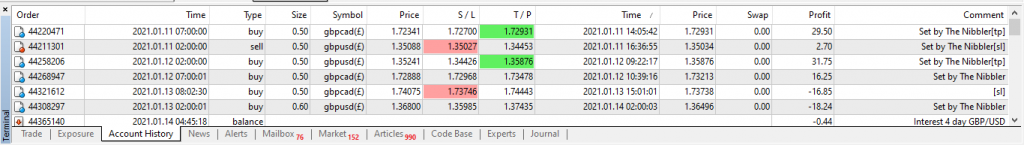
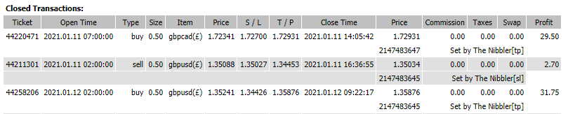
Whilst it is possible to export the Account History for a given time frame, the exported format is an HTML report containing tabular data with trade details spanning multiple rows e.g. the “comment” field, which denotes the MT4 Expert Advisor (a.k.a. trading robot) is in a row below. This makes it difficult to slice and dice the history by robot to understand P&L for each.
How to read the MT4 Account History Report with Jupyter Notebooks
The first thing you need to do is to read the exported statement html file with a Jupyter notebook and convert the tabular data into a pandas dataframe. This uses Beautiful Soup to parse the HTML table.
url = "C:\\Users\\admin\\Desktop\\Statement.htm"
f = open( url , 'r' )
s = f.read()
soup = BeautifulSoup(s)
df = pd.read_html( s )
colNames = ["Ticket", "Open Time", "Type", "Size", "Item", "Open Price", "S / L", "T / P", "Close Time", "Close Price", "Commission", "Taxes", "Swap", "Profit" ]
df[0].columns = colNames
df[0]["Comment"] = ""
df[0]["Magic"] = ""
df[0]["Comment"] = df[0]["Commission"].shift(-1)
df[0]["Magic"] = df[0]["Close Price"].shift(-1)
history = df[0][df[0].Ticket.apply(lambda x: str(x).isnumeric())]
history = history[history["Type"] != "balance"]
history["Open Time"] = pd.to_datetime(history['Open Time'], format = '%Y.%m.%d %H:%M:%S')
history["DOW"] = history["Open Time"].dt.day_name()
history.set_index('Open Time', inplace=True)
history["Profit"] = pd.to_numeric(history["Profit"])
history["CumProfit"] = history["Profit"].cumsum()
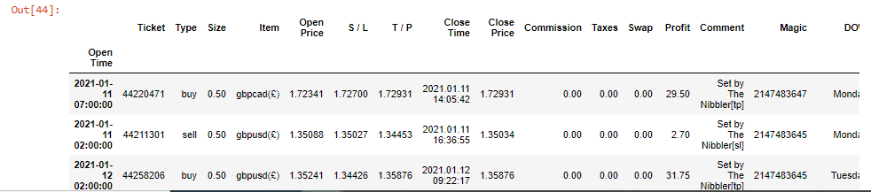
The above code will create a pandas dataframe called history, which contains all columns relevant to your trades. The example also contains a couple of derived columns as an example, e.g. the day of week, and the cumulative profit.
Now we have the dataframe of trade data, we can do whatever we wish. For example if you want to analyze trades by Robot (slice and dice based off the comment field) then simply do the following:
plt.subplots(figsize=(10,6))
history.groupby(['Comment'])["Profit"].sum().sort_values(ascending=True).plot.barh()
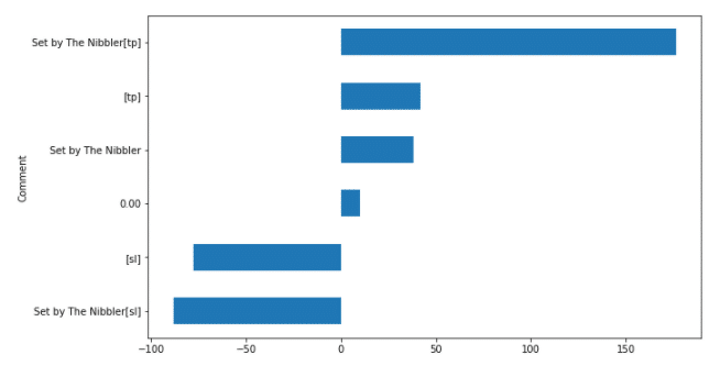
In the example above, “The Nibbler” is a simple trading robot that I created to trade various currency pairs such as GBP/USD. The chart clearly shows P&L for the robot for the timeframe based on when it has hit take-profit (tp) versus stop loss (sl) versus when it was manually closed.
How to find the most profitable currency pair
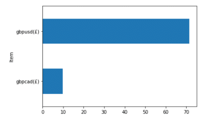
To find the most profitable currency pair for a given trading robot, then you can extract just the rows of the dataframe relevant to that robot (based on a substring of the comment field), and then group based on the “Item” field e.g.
nibblers = history[history["Comment"].str.contains("Nibbler")]
nibblers["CumProfit"] = nibblers["Profit"].cumsum()
nibblers.groupby(['Item'])["Profit"].sum().sort_values(ascending=True).plot.barh()
Other insights I have been able to make using a custom jupyter notbook include:
- Look at Profit and Loss in time series at aggregate, and by each currency pair or trading robot
- Find which currency pairs are most profitable, and modify lot size accordingly
- Find out if there are any particular days when trading is less profitable e.g. I discovered that Friday’s were the worst day for trading
Being able to analyze your trading data in this way allows you to make much better decisions about your future trading strategy, and will hopefully allow you to adapt to make yourself more profitable.


0 Comments